1. Definition of Distance Relay
A distance relay (or impedance relay) is a protection device used on power transmission lines that estimates the distance to a fault by measuring the apparent impedance between the relay location and the fault point. It measures terminal voltage and current, computes the complex quotient \(Z_{app} = \frac{V_R}{I_R}\) and compares it against a preset operating region in the R–X plane. If the measured impedance falls within that region (the reach), and directional criteria are satisfied, the relay issues a trip.
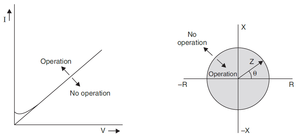
Fig: Operating characteristic of impedance relay on V–I and R–X diagrams
2. Operating principle & phasor basics of Distance Relay
Assume phasor representation for steady‑state conditions. Let the relay measure phase voltage \(V_R=|V_R|\angle\theta_V\) and phase current \(I_R=|I_R|\angle\theta_I\). The apparent impedance is:
\[ Z_{app} \,=\, \frac{V_R}{I_R} \,=\, \frac{|V_R|}{|I_R|} \angle (\theta_V – \theta_I) . \]
For a uniform transmission line of per‑unit length impedance \(z = r + jx\), a fault at distance \(d\) from the relay yields a line impedance to the fault \(Z_{fault}=d\,z = d(r+jx)=d r + j d x\). For an ideal bolted fault (zero fault resistance), the voltage at fault point is (approximately) zero, and:
\[ V_R \approx I_R \cdot d z \quad\Rightarrow\quad Z_{app} \approx d z. \]
Therefore the relay estimates fault distance by:
\[ d \approx \frac{Z_{app}}{z}. \]
3. Formula and derivation (step‑by‑step) of Distance Relay
3.1 Simple line model (series impedance)
Consider a single phase of a transmission line from the relay to the fault point. The line segment of length \(d\) has impedance \(d z\). Writing KVL between relay terminal and fault point:
\[ V_R – V_F = I_R \cdot (d z) , \]
If the fault is bolted and the fault point voltage \(V_F \approx 0\), then \(V_R \approx I_R d z\) and
\[ Z_{app} = \frac{V_R}{I_R} \approx d z. \]
3.2 Including fault resistance
For a fault with finite fault resistance \(R_f\), the voltage drop includes the fault resistance:
\[ V_R = I_R (d z + R_f) \quad\Rightarrow\quad Z_{app} = d z + R_f. \]
This shows that fault resistance adds a real component to the measured impedance: it shifts the point on the R–X plane to the right. Thus a pure reactance‑based relay may be less sensitive to resistive faults while an impedance relay must compensate for this shift.
3.3 Thevenin source and source impedance effect
When the sending network is represented by a Thevenin source \(E_{th}\) with source impedance \(Z_{th}\), the measured terminal voltage is:
\[ V_R = E_{th} – I_R Z_{th} – I_R (d z) – I_R R_f. \]
During a fault the current \(I_R\) depends on \(E_{th}\) and total series impedance seen by the source. Rearranging, the apparent impedance seen by the relay is:
\[ Z_{app} = \frac{V_R}{I_R} = \frac{E_{th}}{I_R} – Z_{th} – d z – R_f. \]
The term \(E_{th}/I_R\) is not simply known a priori and varies with system conditions, so detailed relay reach calculations use system studies and simulation to obtain expected phasor relationships. However, for strong sources where \(Z_{th}\) is small, and when focusing on line contribution, \(Z_{app} \approx d z + R_f\) remains a useful approximation.
3.4 Directional element using complex conjugate
Distance relays must be directional — they should only operate for faults towards the protected line, not for remote faults. A common directional criterion uses the real part of a complex product:
\[ D = \mathrm{Re} \{ V_R \cdot I_R^{*} \cdot K^{*} \} \]
Where \(I_R^{*}\) is the complex conjugate of the current, and \(K\) is a complex polarizing quantity (for example voltage from a remote phase, or the prefault voltage). If \(D > 0\) the direction is forward; if \(D < 0\) it is reverse. In practice modern digital relays implement various directional logic variants (phase, residual, negative‑sequence polarizing).
3.5 Mho characteristic (circle) derivation
Mho (admittance) relays have a circular operating characteristic in the R–X plane. Consider a circle centered at \((R_c,0)\) with radius \(R_c\) so that the circle passes through the origin. The equation is:
\[ (R – R_c)^2 + X^2 = R_c^2. \]
Expanding the left hand side and simplifying gives the mho circle condition:
\[ R^2 + X^2 = 2 R_c R. \]
Replace \(R\) and \(X\) by the real and imaginary parts of \(Z_{app}\) (i.e., \(Z_{app}=R+jX\)). Thus the relay operates if the measured \\(R, X)\\ satisfy the circle inequality inside the radius.
3.6 Quadrilateral characteristic (digital relays)
Modern digital relays commonly use quadrilateral characteristics which are defined by linear inequalities combining \(R\) and \(|X|\). A generic form is:
\[ k_1 R + k_2 |X| \le Z_{reach} , \]
where \(k_1\) and \(k_2\) shape the quadrilateral to be generous in resistive direction (to cover large \(R_f\)) while limiting overreach during remote infeed conditions. The coefficients are chosen based on system studies.
3.7 Reach calculation
If the line impedance per phase (for whole line length \(L\)) is \(Z_{line} = L z = R_{line} + j X_{line}\), and zone‑1 should cover a fraction \(\alpha\) of the line (e.g., \(\alpha=0.8\)), then:
\[ Z_{reach1} = \alpha Z_{line} = \alpha (R_{line} + j X_{line}). \]
Expressed magnitude wise, the reach magnitude is:
\[ |Z_{reach1}| = \alpha \sqrt{R_{line}^2 + X_{line}^2}. \]
4. Types of distance relays
Distance relays can be classified by operating characteristic, measurement method and directionality:
- Mho (admittance) relays: Circular characteristic, inherently directional; fast and used historically in electromechanical forms and in some digital relays.
- Impedance relays: Operate when measured impedance magnitude falls below a threshold (circular/sector style).
- Reactance relays: Respond to the reactance component only (\(X\)); useful for detecting faults with large resistive components avoided.
- Quadrilateral relays: Digital relays that use a four‑sided characteristic to tolerate fault resistance and provide selectivity.
- Directional distance relays: Combine directional elements (phase/residual polarization) with distance elements to ensure forward operation only.
5. Comparison table (types & characteristics)
| Relay Type | Characteristic | Advantages | Limitations |
|---|---|---|---|
| Mho | Circular in R–X (passes through origin) | Directional, simple stability for power swing | Sensitive to fault resistance offset, requires angle compensation |
| Impedance | Operates on |Z| ≤ Z_reach | Intuitive reach setting | Non‑directional unless combined with directional element |
| Reactance | Operates when X ≤ X_threshold | Less affected by R_f | Not suitable beyond certain distances (depends on angle) |
| Quadrilateral | Four‑sided polygon in R–X | Better handling of resistive faults and outfeed | More complex setting process |
6. Advantages & Disadvantages of Distance Relay
Advantages
- Provides selective protection based on fault distance — enables fast clearing of local faults without depending on remote tripping.
- Multiple zones provide graded backup protection for adjacent lines and system security.
- Directionality and pilot schemes enhance security and sensitivity.
Disadvantages
- Fault resistance, CT saturation, source impedance and power swings can cause maloperation or underreach/overreach; requires careful settings and compensation.
- Complexity in settings — requires system studies, relay coordination and sometimes pilot communication.
- Older electromechanical relays had limited ability to handle resistive faults but digital relays improved this.
7. Applications of Distance Relay
- Transmission line protection (EHV/HV): primary use is selective tripping of faulty line sections.
- Zone backup protection for generator feeders and interconnects.
- Used in pilot protection schemes (e.g., directional comparison, permissive overreach) to increase selectivity and reduce incorrect tripping.
- Reactive power and stability monitoring as part of advanced protection schemes.
8. Worked example (numerical)
Given a line: length \(L=100\,\mathrm{km}\), per‑km impedance \(z=0.1 + j0.4\,\Omega/\mathrm{km}\). Compute zone‑1 reach for \(\alpha=0.8\).
Line impedance:
\[ Z_{line} = L z = 100(0.1 + j0.4)=10 + j40\,\Omega. \]
Zone‑1 reach:
\[ Z_{reach1} = \alpha Z_{line} = 0.8(10 + j40) = 8 + j32\,\Omega. \]
Magnitude:
\[ |Z_{reach1}| = \sqrt{8^2 + 32^2} = \sqrt{64 + 1024} = \sqrt{1088} \approx 32.98\,\Omega. \]